Use case WF 1
Relationship between primary productivity and temperature in the marine environment
The case study investigates how Primary Production (PP) is influenced by variability in Sea Surface Temperature (SST) and chlorophyll-a (Chl-a). It is based on an integrated framework that combines in situ ocean observations, satellite remote sensing data, and regression machine learning techniques to explore the links between these key variables.
This approach makes it possible to analyse how SST-driven changes propagate through phytoplankton dynamics to influence PP over long periods. Ultimately, the study aims to improve our understanding of the response of marine ecosystems to climate-driven changes in ocean temperature and to provide more robust information on the evolution of oceanic primary production in a warming climate.
Dataset
The dataset used for this case study was derived from field measurements available on the Ocean Productivity website. The oceanographic dataset includes water temperature, chlorophyll-a concentration, and primary productivity estimates obtained using the ¹⁴C method. For this analysis, we selected measurements taken at the sea surface within the equatorial zone. Further details on the original data types and processing methods are available at:https://orca.science.oregonstate.edu/field.data.c14.online.php
The dataset also includes sea surface temperature and chlorophyll-a concentration, derived from Ocean Color’s remote sensing imagery, at an 8-day temporal resolution (https://oceandata.sci.gsfc.nasa.gov/l3/). In particular, the WF offers the ability to download various ocean colour products directly from the virtual research environment. Additional details about the dataset used in this use case are publicly available through the LifeWatch Italy metadata catalogue at the following link: https://metadatacatalogue.lifewatchitaly.eu/geonetwork/srv/eng/catalog.search#/metadata/811ebcbd-b85d-4e5a-871f-5b3afa44f712
Method
The aim of this study is to develop an advanced analytical framework with which to understand the dynamics of Primary Production (PP) in relation to variability in Sea Surface Temperature (SST) and chlorophyll-a (Chl-a). The framework integrates in situ ocean measurements, remote sensing imagery and machine learning techniques to investigate the relationships between these key variables.
The methodology consists of the following main steps:
- Regression model development: Linear regression and Random Forest models were implemented to estimate PP using Chl-a and SST variables derived from field-based oceanographic data.
- Application of the regression model to satellite data: The model with the best performance was applied to a selected portion of the study area using 8-day Chl-a concentration and SST imagery derived from MODIS. This produced a new PP image product covering the period from 2004 to the end of 2023.
- Statistical analysis of time series: Statistical analyses were carried out on the SST, Chl-a and PP datasets to compute mean time series for each variable, and to assess temporal trends using the Kendall test, which identifies the direction and statistical significance of trends.
- Recurrence plot analysis: Recurrence plot analysis was applied to the SST, Chl-a and PP time series to investigate short-term variability and detect potential perturbations or regime shifts over time.
- Forecasting future scenarios: A SARIMAX model was implemented to forecast future PP dynamics in relation to Chl-a and SST. This provided possible future scenarios of primary production under varying oceanographic conditions.
Results
Regression Model Estimation
The models were trained and evaluated using cross-validation to limit overfitting and obtain a robust estimate of their predictive ability. This procedure allowed for a reliable assessment of model performance and their ability to generalize to independent data. The models were developed using a logarithmic transformation (ln) applied to the entire dataset. The results show that, in our case study, the Random Forest algorithm outperformed the Linear Model in predicting PP from Chl-a and SST (Table 1). Specifically, the Random Forest model achieved the highest R² and the lowest MAE and RMSE values, confirming its superior ability to capture variability in the dataset and to provide more accurate PP estimates with fewer prediction errors.
Table 1. Evaluation of the regression and random forest model accuracy and performance.

Time series analysis of SST, Chl-a
The portion of the study area was extracted from each 8-day SST and Chl-a remote sensing image. For each 8-day image, the mean value of each variable was calculated to construct a time series of SST and Chl-a of the study area. A spline was applied to the time series derived for SST, Chl-a, to obtain a trend that visually describes the temporal evolution of each series (Figure 1).
Figure 1a illustrates the time series of mean Chl-a, which is characterised by high short-term variability and a weak long-term trend. The smoothing spline curve highlights a slight decrease until the mid-2010s, followed by an increase in more recent years.
Figure 1b displays the time series of mean SST, which exhibits a pronounced seasonal cycle superimposed on a long-term trend that is more regular than that observed for Chl-a. The smoothing spline indicates a gradual temperature increase from the mid-2000s to 2018–2020, followed by a slight decline in subsequent years.
For the missing scenes Chl_2022_0407_2022_0414 and SST_2018_0101_2018_0108, the gap created in the time series was filled by replacing the missing values with the average of the observations immediately before and after each gap.

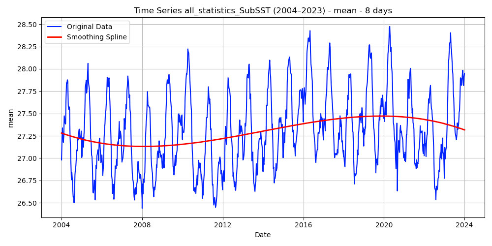
Figure 1. Temporal evolution of Chl-a (a) and SST (b) over the period 2004–2023, using 8-day composites.
The long-term trend analysis based on the Kendall test and the Theil–Sen estimator revealed markedly different behaviours between SST and Chl-a. For SST, a statistically significant increasing trend was detected (τ = 0.1594, p = 4.47×10⁻¹³), with a positive slope estimated by the Theil–Sen method (0.000598). This result confirms a monotonic increase in temperature over the study period, consistent with warming signals reported for many marine regions globally. In contrast, the Chl-a series does not show any significant trend (τ = –0.0149, p = 0.4997), and the estimated slope is near zero (–8.5×10⁻⁷). This indicates that, despite substantial intra- and interannual variability, no persistent direction of change emerges.
The relationship between Chl-a and SST was analysed by computing the Pearson correlation coefficient for each pair of temporal images covering the study area for all time series. The results indicate a scenario characterised by generally weak and predominantly negative correlations between the two variables. The distribution of correlation coefficients shows moderate variability, with values ranging from a minimum of –0.175 to a maximum of 0.087. However, the inverse relationship between Chl-a and SST, although weak, is a persistent feature of the system rather than the result of individual events or seasonal anomalies.
Recurrence Plot Analysis
Recurrence plots (RPs) computed for SST and Chl-a reveal markedly different recurring structures between the two series, highlighting the dynamic and complex nature of the oceanographic processes involved. The SST series RP displays a highly organised structure characterised by regular diagonal patterns reflecting a strong cyclical component and an almost periodic dynamic (Figure 2a). In contrast, the Chl-a series exhibits a much more disordered RP with fragmented patterns that lack a dominant recurring structure (Figure 2b).
In addition to providing information on the system’s cyclicity, RPs also allow potential disturbance events to be identified. The Chl-a RP shows interruptions to the diagonal structures, areas of low recurrence and irregular patterns arranged in ‘patches’ or short vertical or horizontal bands. These features are indicative of phases in which the system’s trajectory in phase space temporarily deviates from its ‘average’ seasonal state, potentially representing signatures of episodic disturbance events (e.g. extreme meteorological conditions, intense mixing episodes, thermal anomalies, or abrupt changes in nutrient availability).
While the RP cannot identify the specific nature of individual events, analysis indicates that the seasonal regime is frequently modulated by disturbance episodes that interrupt the system’s quasi-periodic dynamics.
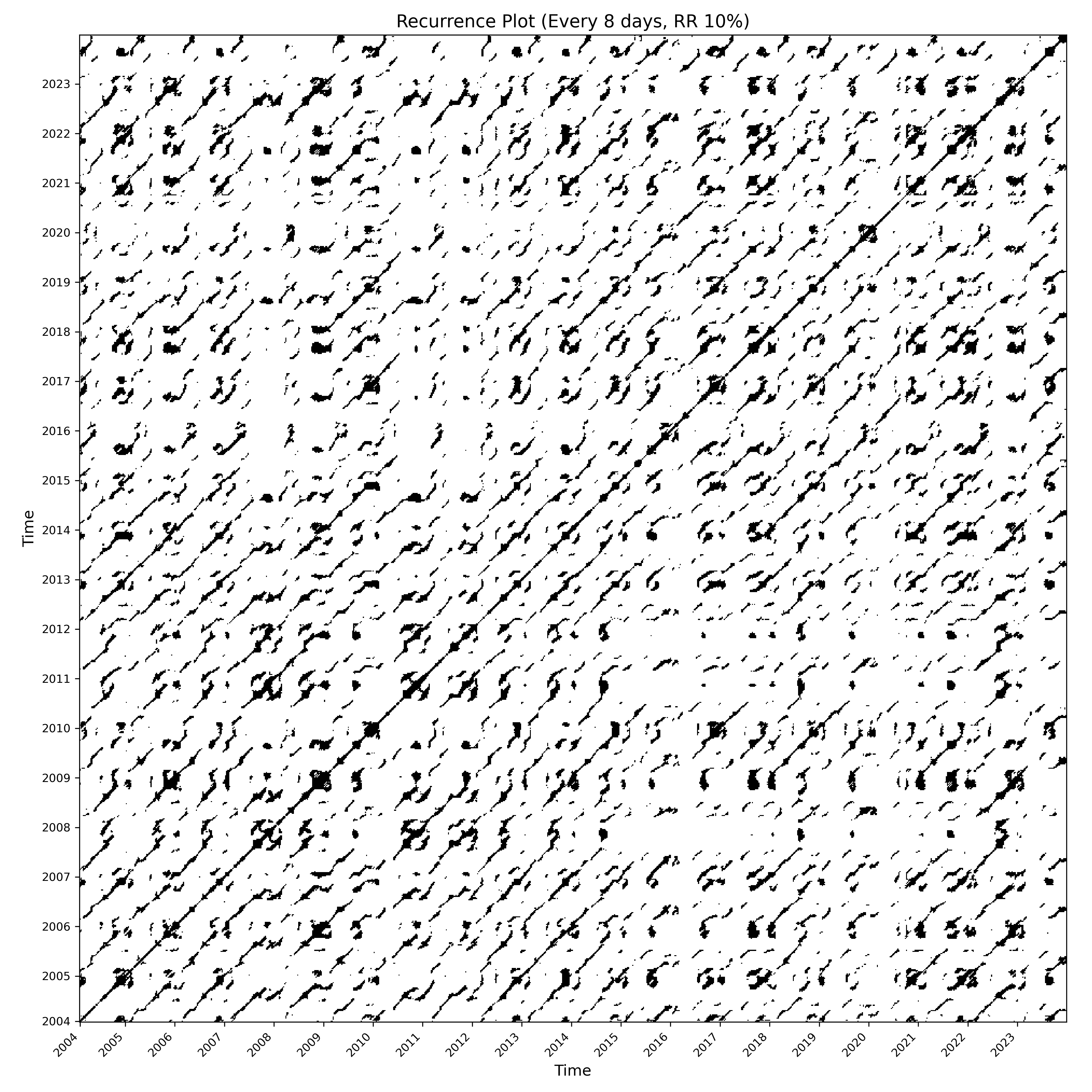
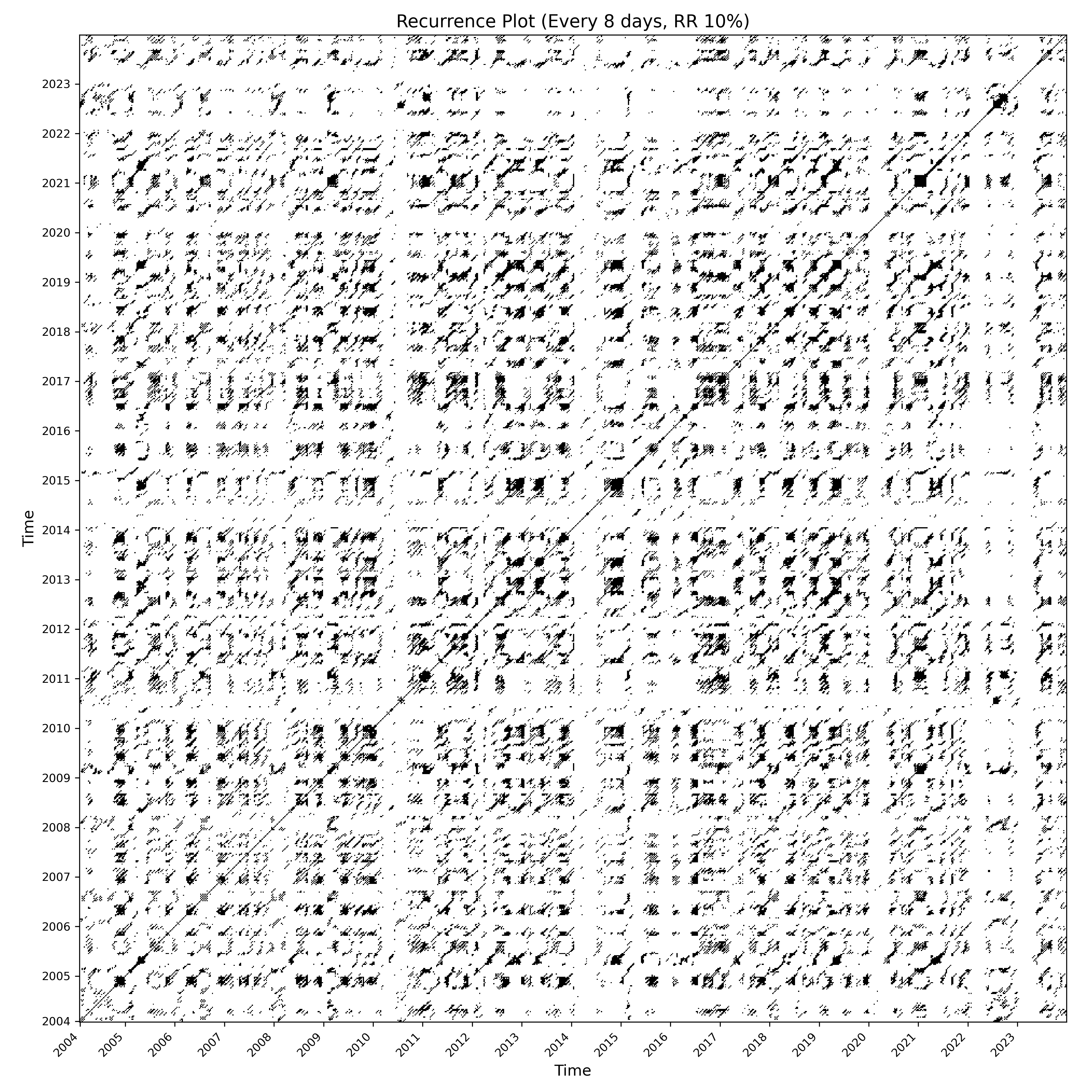
Figure 2. Comparison between two recurrence plots constructed using data sampled every 8 days. a) Recurrence plot for the SST time series. b) Recurrence plot for the Chl time series.
Estimation of PP time series
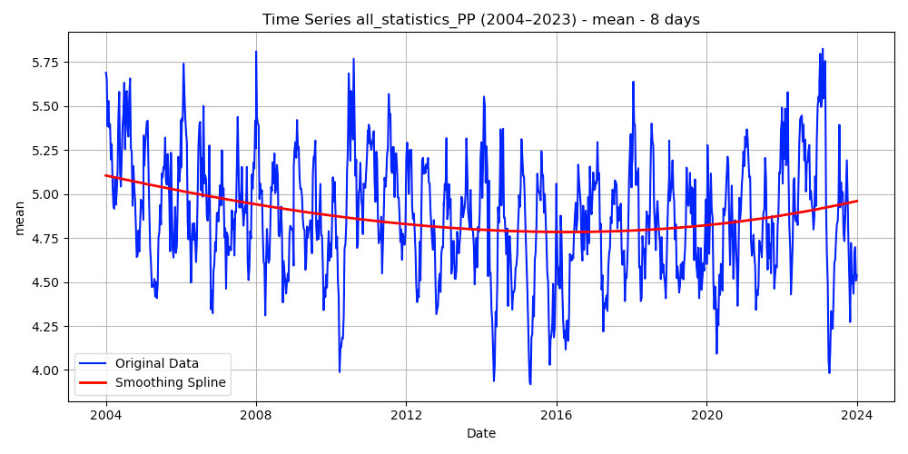
The Random Forest model was then used to predict PP using the 8-day Chl-a and SST images for the study area from 2004 to 2023. Since the Random Forest had been trained on log-transformed data, the same logarithmic transformations were applied to the imagery to ensure consistency with the model configuration. A spline was applied to the time series derived for PP to obtain a trend that visually describes the temporal evolution of PP (Figure 3).
Figure 3 shows the time series of mean primary productivity (PP) for the period 2004–2023, computed using 8-day composites. The series is characterized by marked short-term variability, with regular oscillations that reflect the seasonal dynamics of the system. The smoothing spline curve highlights a weak long-term trend: after relatively higher values in the early part of the series, a slight decrease is observed up to around the mid-2010s, followed by a partial increase in more recent years.
Analysis of the long-term trend in PP, conducted using the Kendall test and the Theil–Sen estimator, reveals statistically significant behaviour over the examined period. The Kendall coefficient (τ = –0.1029, p = 2.98×10⁻⁶) indicates a monotonic decrease, which is further confirmed by the negative slope estimated using the Theil–Sen method (–0.0002245).
Future development scenario of PP
Most climate-change projections focus on long time horizons (50–100 years), whereas in this work we provide a short-term forecast (5 years). The SARIMAX model for PP was developed using SST and Chl-a as exogenous predictors, projected forward in time to support near-term estimates of PP. A 16-day temporal resolution was adopted, since the 8-day frequency did not yield stable or statistically reliable forecasts (Figure 4a).
Diagnostic checks indicate a good model fit: residuals are centred around zero, show no evident temporal structure, and display an approximately symmetric, only slightly platykurtic distribution (Figure 4b and Figure 4c). The Ljung–Box test confirms the absence of significant residual autocorrelation (p > 0.05), suggesting that temporal dependence is adequately captured.
The forecasts indicate that, in the coming years, primary productivity will maintain a seasonal pattern similar to that historically observed. No marked trends or signals of structural changes emerge within the forecast period, suggesting a relative stability of the system in the medium term. Seasonal oscillations remain well defined, and the amplitude of variability falls within the limits of past fluctuations; the 95% confidence intervals remain relatively narrow, supporting the reliability of the forecasts. In the absence of anomalous external forcing, the projections suggest that PP will continue to oscillate within historical ranges, with no evidence of substantial increases or decreases over the period considered.
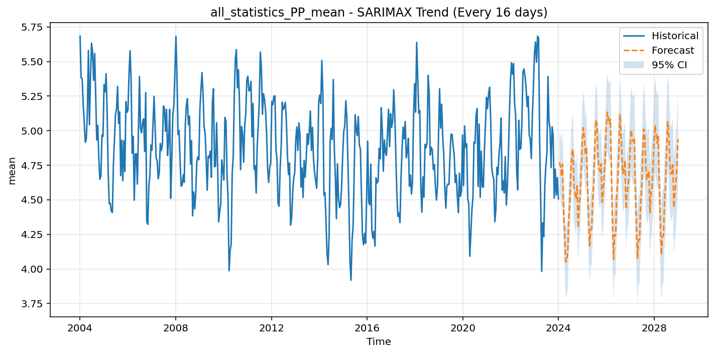

Figure 4. a) Time series of mean primary productivity (PP) and 5-year forecast obtained using the SARIMAX model (16-day resolution), with 95% confidence interval. b) Model residuals, showing no evident temporal patterns. c) Distribution of the residuals, approximately symmetric and centered around zero, confirming the good adequacy of the model.
Technical Notes
The analysis performed illustrates the methodology that can be developed using WF1. The analysis carried out in this case study was naturally set up according to the information available in the dataset used for training and validating the regression model. However, the workflow is designed to work with any tabular dataset in which variables and factors are reported in columns. The important thing is the right setting of the Parameter data file. Therefore, analyses can be configured based on specific datasets provided by users and their analytical needs. The main analyses can be configured according to the specific case study that the user wants to develop.
In this work, PP data were used, but the user can also employ other types of data, such as biomass concentrations and other biotic parameters from field monitoring, which can be consistently compared with the available satellite image datasets.