Use case WF 3
Influence of behavioral and functional traits on the home range-body mass relationships in consumer species
Body size and home range are fundamental attributes that reflect the energetic demands, locomotor capacity and spatial strategies of consumer species. Allometric and movement ecology theories predict a positive allometric scaling of home range with body mass. Nevertheless, the strength and functional form of this scaling can vary widely among taxa as a result of differences in behavioural, ecological, and physiological traits. For instance, aquatic and terrestrial species encounter distinct spatial and environmental constraints that can shape their movement patterns and space-use strategies. Primary diet may further influence home-range size through contrasts in foraging ecology, dietary energy content, and resource distribution. Locomotion mode also affects movement efficiency and the energetic costs associated with space use. Similarly, the thermoregulatory strategy of organisms (endothermy vs ectothermy) influences metabolic rates and the allocation of energy to movement and resource acquisition. All these variables, may hence potentially influence the home range-body mass relationship.
Using a trait-annotated species database that includes information on habitat, primary diet, thermoregulatory strategy, and locomotion mode, the analytical workflow tests the home range-body mass scaling relationships within each trait class and evaluates between-groups differences in scaling parameters. This approach allows the user to visualize and assess how functional and behavioural traits mediate space-use patterns across vertebrate taxa and to test whether these traits systematically modify fundamental allometric expectations.
This case study, as a part of WF3, focuses on testing various analytical operations on a designed dataset describing the behavioural and functional traits of vertebrate species, with the specific aim of assessing how these traits influence the relationship between home-range and body mass. It should be noted that, within the same workflow, users may perform different or additional analyses involving other variables, depending on the structure and content of their own input files. In addition, users may perform similar operations by importing an individual-level dataset of the same species, including other categorical variables for specific tests. The dataset reported below is therefore provided as an example.
Dataset
The provisional dataset includes behavioural and life-history traits for a representative selection of aquatic and terrestrial vertebrate species compiled from the published literature. Estimates of home-range size and body mass were gathered from three primary sources: Tamburello et al. (2015), McCauley et al. (2015), and Udyawer et al. (2023). These datasets were merged into a single harmonised dataset. For species represented in more than one source, home-range values (expressed in m²) and body-mass values (expressed in g) were averaged to obtain a single estimate per species. The resulting dataset comprises 1,164 species-level records, spanning fishes (n = 191, including elasmobranchs), reptiles (n = 136), mammals (n = 642), and birds (n = 195) from across the globe.
For each species, the following key parameters were compiled: body mass (bodyMass) and home-range area (meanHomeRange), both treated as numerical variables. In addition, several categorical traits were included: habitat (terrestrial or aquatic), thermoregulatory strategy (endothermic or ectothermic), primary locomotion mode (walking, swimming, flying, crawling), and primary food type (carnivore or herbivore). These trait data were obtained from published sources and associated datasets. Additional details about the dataset used in this use case are publicly available through the LifeWatch Italy metadata catalogue at the following link: https://metadatacatalogue.lifewatchitaly.eu/geonetwork/srv/eng/catalog.search#/metadata/32b7709b-88a1-4768-a6ee-e98aec7f813f.
Methods
The analysis was conducted on the entire dataset, after applying a logarithmic transformation (log10(x)) to all numeric variables. The analysis was performed by setting meanHomeRange as the dependent variable (Y) and bodyMass as the independent variable (X), to assess the presence and strength of linear relationship between the two. Model specifications were provided in a configuration file (Parameter.csv), which enabled the automatic distinction between regression and analysis of covariance (ANCOVA) analyses. The ANCOVA models incorporated additional categorical predictors (trait variables), enabling the evaluation of how behavioural and functional traits influence the home range-body mass relationship.
A schematic summary of the analytical steps is provided below:
- Regression model:
- Dependent variable (Y):
- Covariate (X): bodyMass (this variable was mean-centered).
- ANCOVA model:
- Dependent variable (Y):
- Covariate (X): bodyMass (this variable was mean-centered).
- Factors (f): habitat, thermoregulation, locomotion,
This framework enables the assessment of variation in meanHomeRange as a function of bodyMass , while accounting for differences associated with habitat and other ecological or behavioural traits.
The data regression and ANCOVA analysis were performed using linear models implemented in Python (the statsmodels package). Prior to model fitting, continuous covariates were mean-centred to facilitate interpretation of the main effects in the presence of interactions. A full ordinary least squares (OLS) model was then estimated, including all main effects of covariates and factors, as well as all covariate × factor interactions in ANCOVA analysis. Sum-to-zero (Sum) contrasts were applied to categorical factors and estimates were computed with robust standard errors (HC3). Factors with only one observed level were automatically excluded. The final model was selected using a backward selection procedure within an information-theoretic framework. Terms were iteratively dropped, while preserving the hierarchy between main effects and interactions, until the AIC improved. During this process, multicollinearity constraints were enforced using the variance inflation factor (VIF< 3), with terms having VIF values above a predefined threshold being removed. Residual diagnostics were conducted for both the full and final models, together with Shapiro-Wilk tests for normality and Breusch-Pagan tests for heteroskedasticity. Inference on effects was summarised using Type III ANCOVA tables, with effect sizes expressed as partial η². For each retained factor, estimated marginal means (EMMs/LS-means) were computed with Holm-adjusted pairwise comparisons. Finally, regression lines for key covariates and ANCOVA lines, stratified by factor levels, were plotted, including 95% confidence intervals.
Dataset transformation
At this stage, a check is performed for non-values, and if any are found, they are removed. In addition, species for which the original value equal 1 were removed, as this would result in zero after the log transformation. After these steps, the final dataset used for the analyses consisted of 1,162 species (configurable action). These filters can be adjusted by the user according to specific analytical needs.
Results
Linear regression: the relationship between home range and body mass.
Regression analysis confirmed a positive and highly significant relationship between mean home range size and body mass. The model explains a substantial proportion of the observed variation in mean home range (R² = 0.557) and indicates that a one-unit increase in centred body mass is associated, on average, with a 1.24-unit increase in home-range size (β = 1.2419, p < 0.001).
The nearly perfect linear relationship between the observed and fitted values further illustrates model fit, suggesting high consistency between the model and the data (Figure 1). However, inspection of the residuals reveals some deviations from the assumptions of a classical linear model. The diagnostic deviations may reflect extreme values that are biologically meaningful (e.g. ecologically atypical species) or an inherently skewed distribution of home-range sizes across taxa within the dataset. This finding is consistent with the Shapiro-Wilk test, which strongly rejects the null hypothesis of normality (p = 5.3 × 10⁻¹⁶). The Breusch-Pagan test also revealed significant heteroskedasticity (p = 0.036), suggesting that the variance of the residuals increases with the fitted values. To address this, HC3 heteroskedasticity-robust standard errors were employed, confirming the significance and robustness of the estimated coefficients.
Overall, the model demonstrates a strong fit and a robust effect of body mass on home range size. This indicates that body mass is a strong predictor of home-range size. Nonetheless, additional ecological and behavioural variables may contribute to variation in home-range size across species, accounting for part of the unexplained variation beyond body mass alone.

ANCOVA – pairwise comparison
Subsequent ANCOVA analysis incorporating additional categorical factors as fixed effects, were conducted to evaluate the extent to which behavioural and ecological traits influence both the intercepts (mean body mass at a given home range) and the slopes (body mass scaling). This approach allows for the separation of general allometric patterns from functional differences among ecological groups. It is important to note that, at this stage, the user can choose to include or exclude one or more fixed factors when running the model, depending on the research questions and the relationships among the variables.
In detail: To examine the relationship between home range and body mass more thoroughly, we considered four categorical factors that could potentially modulate this relationship. A factorial analysis was conducted, incorporating either all factors or a selected subset, depending on the degree of multicollinearity observed among the variables and their interaction terms.
The global model, which included all main effects and their interactions, demonstrated strong explanatory power (R² = 0.754; adj. R² = 0.751). Body mass, locomotion type, thermoregulation strategy, and primary diet significantly influence mean home range across species. Flying animals and carnivores also exhibit larger mean home ranges. Some predictors, such as aquatic habitat and swimming locomotion, were not statistically significant. Overall, the results highlight the combined effect of body mass, ecological traits, and interactions on home range size. However, residual diagnostics indicate moderate skewness and kurtosis. The residuals significantly deviated from normality (Shapiro-Wilk p = 3.6 x 10⁻¹⁴) and strong heteroskedasticity was evident (Breusch-Pagan p = 3.7 x 10⁻¹5), and standard errors were corrected for heteroscedasticity (HC3). The very small eigenvalue suggests potential multicollinearity in the model, which should be considered when interpreting coefficients.
Consequently, the analysis proceeded with a model simplification strategy. Non-significant predictors and interactions were systematically removed, guided by information criteria (AIC) and multicollinearity checks (VIF < 3), to obtain a more parsimonious model that retains explanatory power while satisfying classical linear model assumptions.
The selected model, derived through AIC-based model selection and VIF filtering, indicates that body mass, thermoregulation strategy, and primary diet were significant predictors of mean home range. As expected, its explanatory power is slightly lower, approximately 68% (R² = 0.685; adjusted R² = 0.683), but the model is more parsimonious and its coefficients are more stable. Ectothermic species tend to have smaller home ranges, while carnivores have larger ones, with body mass amplifying these effects. Diagnostic tests still indicate deviations from residual normality (Shapiro-Wilk p = 7.7 x 10⁻¹8) and persistent heteroskedasticity (Breusch-Pagan p = 1.9 x 10⁻⁶), although these issues are less pronounced compared to the global model.
Panels in Figure 2, compare effects from the global and selected model (Figure 2). The selected model represents a more balanced compromise between complexity, coefficient significance, and statistical parsimony. Although it does not fully resolve the issues related to the error structure, it reduces the over-specification of the full model and is preferable in terms of interpretability and inferential stability. Overall, this finding supports the notion that body mass is the primary determinant of home-range size, while its effect on space use may be modulated by other key biological traits.
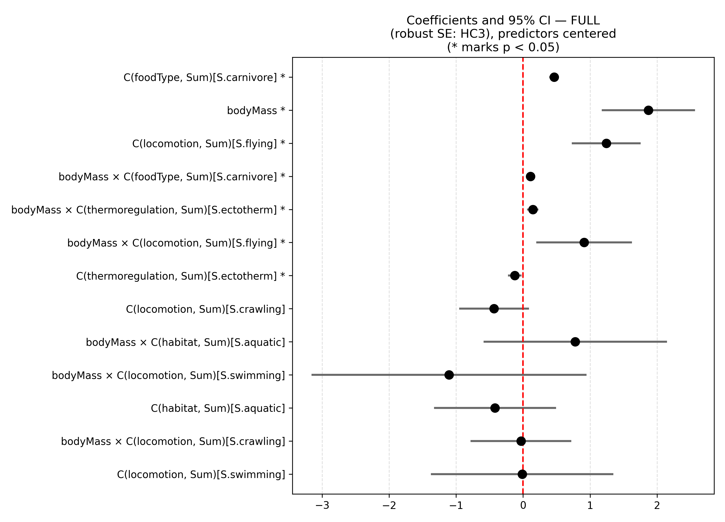
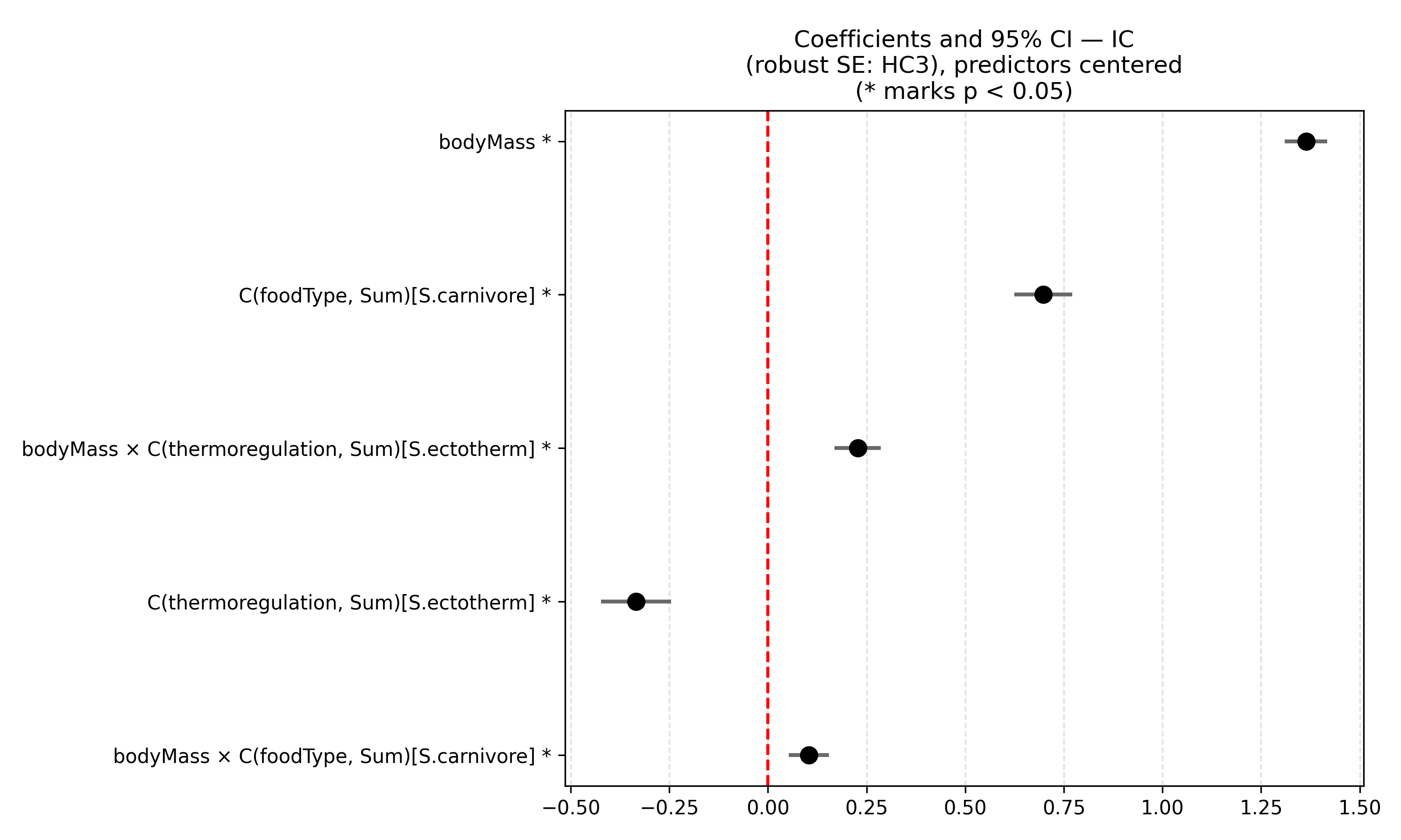
Figure 2: The two panels show the estimated coefficients (with 95% confidence intervals and robust standard errors, HC3) for the global model (a) and the model selected using information criteria with multicollinearity control (b).
In summary, the ANCOVA model for the selected specification (after applying the VIF criterion) identified body mass as the strongest predictor of home-range size, with a positive and highly significant effect across all taxonomic and ecological groups considered. Two categorical factors, thermoregulatory strategy and primary food type, showed significant main effects as well as significant interactions with body mass. This indicates that the relationship between body mass and space use is not uniform across groups.
A similar pattern emerges for the food type predictor (Figure 3a): carnivores consistently show larger home ranges than herbivores, along with a steeper scaling with body mass. This interaction suggests that trophic ecology modulates the allometric relationship between body mass and space use.
As shown in Figure 3b ectotherms exhibit a steeper relationship between home-range size and body mass compared to endotherms, suggesting that increases in body mass translate into proportionally greater spatial requirements in ectothermic species. Post-hoc analyses on the estimated marginal means (Holm correction) confirm significant differences between the two groups, particularly at intermediate and high body-mass values (Figure 4).
Overall, the ANCOVA results suggest that body mass is the principal determinant influencing home-range size. However, the exact relationship between the two depends strongly on the species’ thermal and trophic ecology.


Figure 3. The plots show the relationships between body mass and home-range size in the selected models, highlighting how these relationships vary according to food type (a) and thermoregulatory system (b). In both cases, home-range size increases with body mass, but systematic differences emerge between groups.
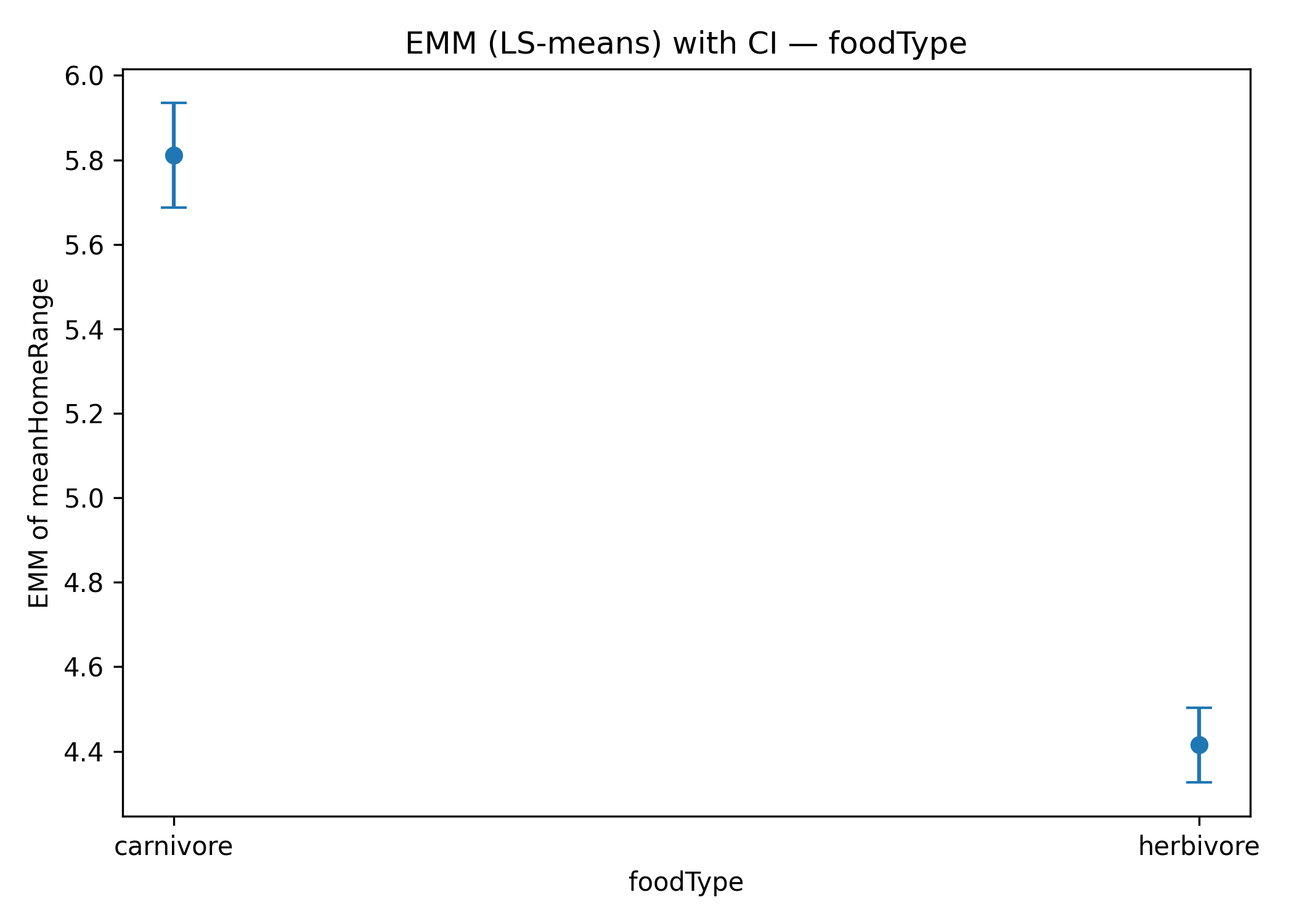
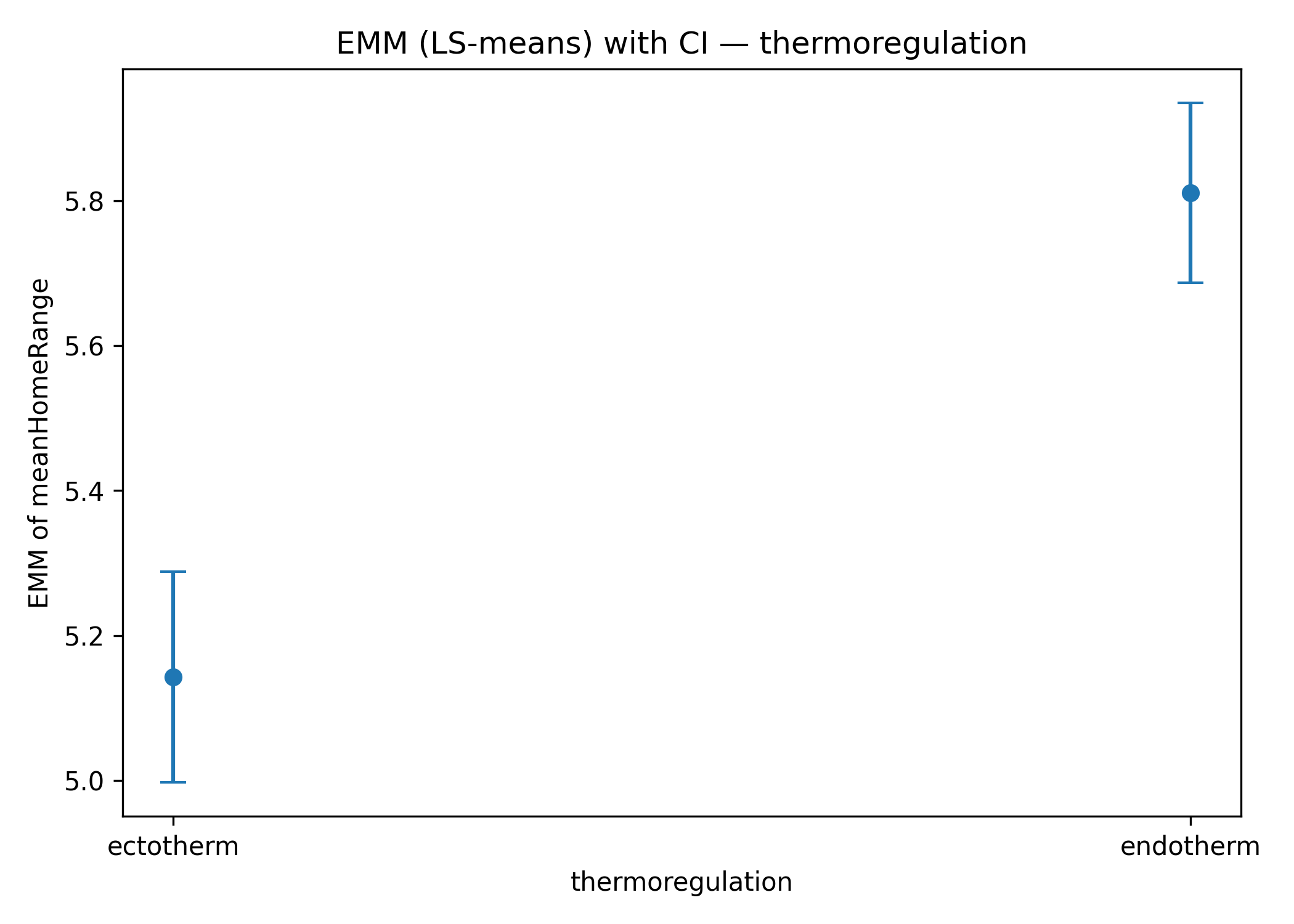
Figure 4: Estimated marginal means (EMMs) for categorical predictors: a) foodType: carnivores vs herbivores; b) thermoregulation: ectotherms vs endotherm.
Technical Notes
The analysis presented here demonstrates the methodology that can be implemented using WF3. In this case, the analysis was structured according to the information available in the dataset. However, the workflow is designed to accommodate any tabular dataset in which variables and factors are organized in columns. Analyses can thus be tailored to the specific structure of user-provided datasets and the corresponding research questions. Notably, exact column names are not mandatory. The system can be configured using different covariate settings (X) in the Parameter.csv file. The important point is that the header of the Parameter.csv file used to configure the analysis corresponds to the headers in the input table. Furthermore, the workflow offers several configuration options for regression and ANCOVA analyses, providing considerable flexibility to meet individual user needs.