Use case WF 4
Application of machine learning models for ecological analysis
Workflow 4 (WF4) aims to evaluate a range of machine learning algorithms that can be adapted to different ecological problems. The goal is to identify the most suitable model for analysing the influence of predictor variables on a target variable. Designed with a pragmatic approach, the workflow is applicable across a wide spectrum of climate-change-related scientific domains, particularly regression analyses. Currently, WF4 supports regression modelling on any dataset of biotic and abiotic variables (characterised by a numerical variables), identifying key relationships based on user goals, available data and parameter settings.
The proposed case study showcases WF4’s core capabilities. Using the selected dataset, it examines on the relationship between Primary Productivity (PP) and biotic variables such as chlorophyll concentration (Chl), as well as abiotic variables including sampling month (month), latitude (decimalLatitude), longitude (decimalLongitude), distance from the coast (distanceFromCoast, irradiance (Irr), day length (dayLength), and sea surface temperature (SST).
Dataset
The dataset used for this case study was derived from field data available on the Ocean Productivity website. We selected measurements taken at the sea surface (depth = 0 m). We created the dataset by adding the distance of each monitoring site from the coast, calculated using the geographic coordinates provided in the original data. Further details on the original data types can be found at: https://orca.science.oregonstate.edu/field.data.c14.online.php. Additional details about the dataset used in this use case are publicly available through the LifeWatch Italy metadata catalogue at the following link: https://metadatacatalogue.lifewatchitaly.eu/geonetwork/srv/eng/catalog.search#/metadata/811ebcbd-b85d-4e5a-871f-5b3afa44f712
Methods
WF4 simultaneously evaluates five machine-learning regression algorithms, as eXtreme Gradient Boosting (XGBoost), Multiple Linear Regression, Neural Networks, Random Forests and Support Vector Machines, to identify the algorithm that best captures the relationships under study. In this case study, the goal was to estimate how PP (settled in this study as target variable in the “Parameter data” file) is influenced by the available biotic and abiotic variables (the predictors present in the input table “Training data” file).
In this case study, model selection is based on the Mean Absolute Error (MAE) by default. However, this can be configured in the ‘Parameter data’ file, and the best model can be chosen using the Root Mean Squared Error (RMSE) or the coefficient of determination (R²).
Models are trained using cross-validation and then tested on a dataset that has been held back. Before training begins, WF4 can optionally apply data transformation pipelines. In this study, we train the model using data preprocessed through normalization and principal component analysis (PCA). The original dataset is automatically split into training and test sets according to the specifications provided by the user in the ‘Parameter data’ file. The trained algorithm is then applied to the test set to evaluate its ability to generalise to new data.
Hyperparameters are defined as ranges or candidate values in the “Parameter data” file. WF4 explores these and selects the combination that yields the best performance for the chosen evaluation metric.
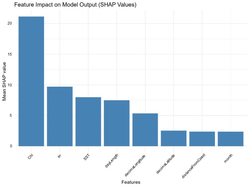
Finally, WF4 runs a SHAP (SHapley Additive exPlanations) analysis on the best-performing model to identify which variables most strongly influence model behavior.
Results
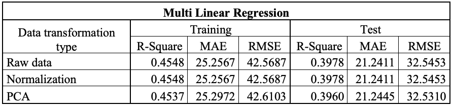
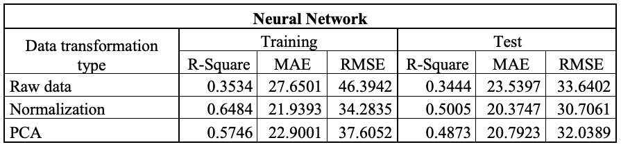
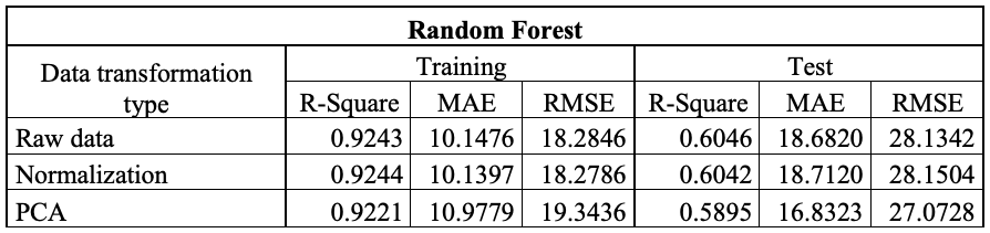
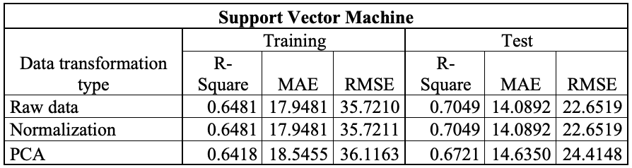
The Table 1 report R², MAE and RMSE for the training and testing phases for the algorithms, using both raw and transformed data. In this case study, normalization and PCA were applied to the data (Full results are provided in the ‘model_parameters_description’ file in the folder of each model). Using the chosen approach, eXtreme Gradient Boosting (XGBoost) achieves the lowest MAE in the training phase when trained on raw data (Table 1A). In the testing phase, however, the Support Vector Machine (SVM) is the best-performing algorithm when trained on raw data (Table1B).
Table 1. Tables reporting the performance results of the applied models. a) eXtreme Gradient Boosting; b) Multi Linear Regression; c) Neural Network; d) Random Forest and e) Support Vector Machine.
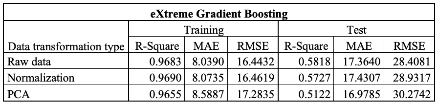
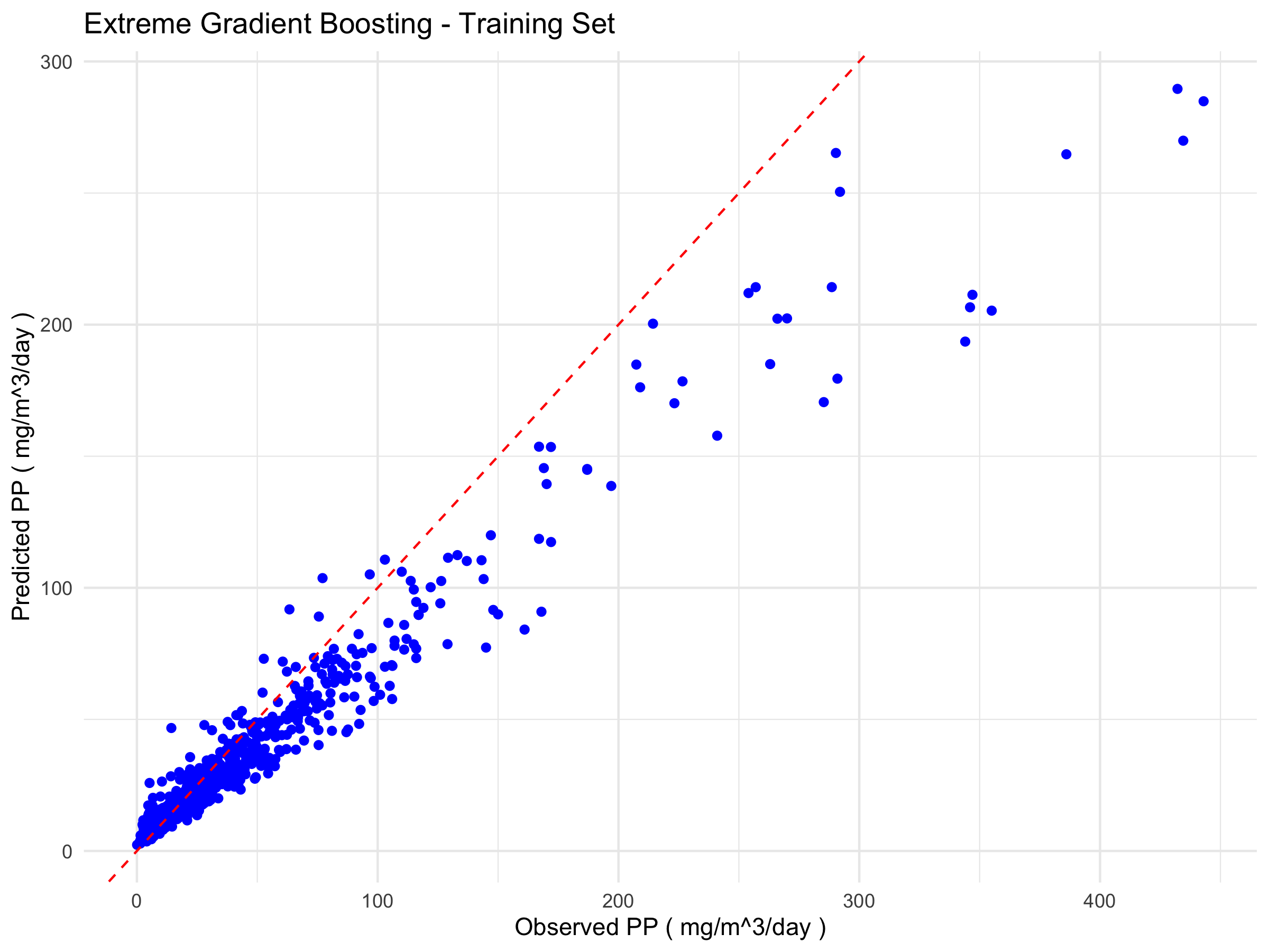
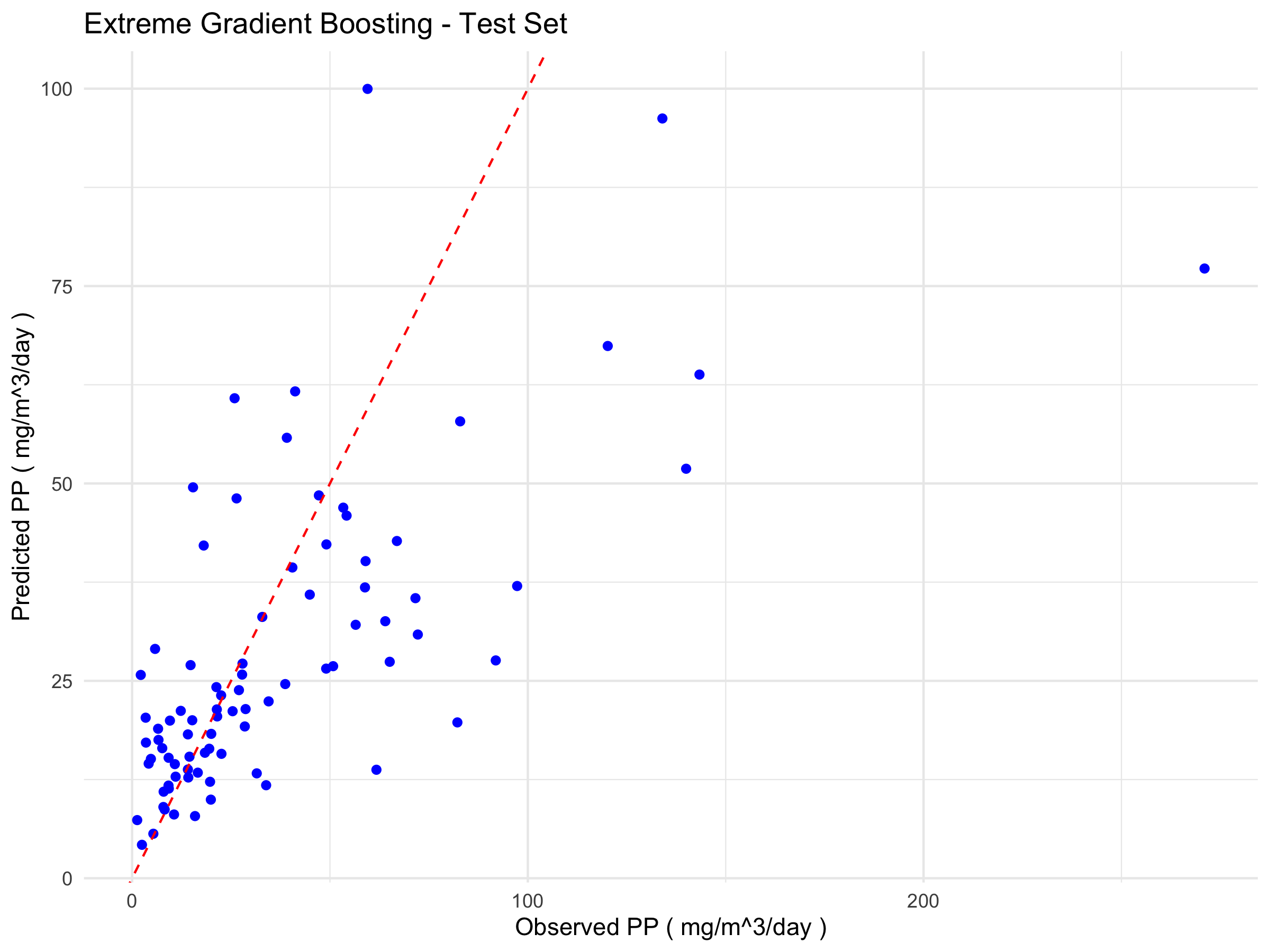
A comparative analysis of the eXtreme Gradient Boosting (XGBoost) and Support Vector Machine (SVM) models reveals notable differences in their generalisation capabilities. While XGBoost performs excellently on the training set (R² = 0.9683), it shows a marked decline on the test set (R² = 0.5818), accompanied by substantial increases in MAE and RMSE. This behaviour indicates overfitting, whereby the model learns the characteristics of the training set too specifically, thereby compromising its ability to predict unseen data.
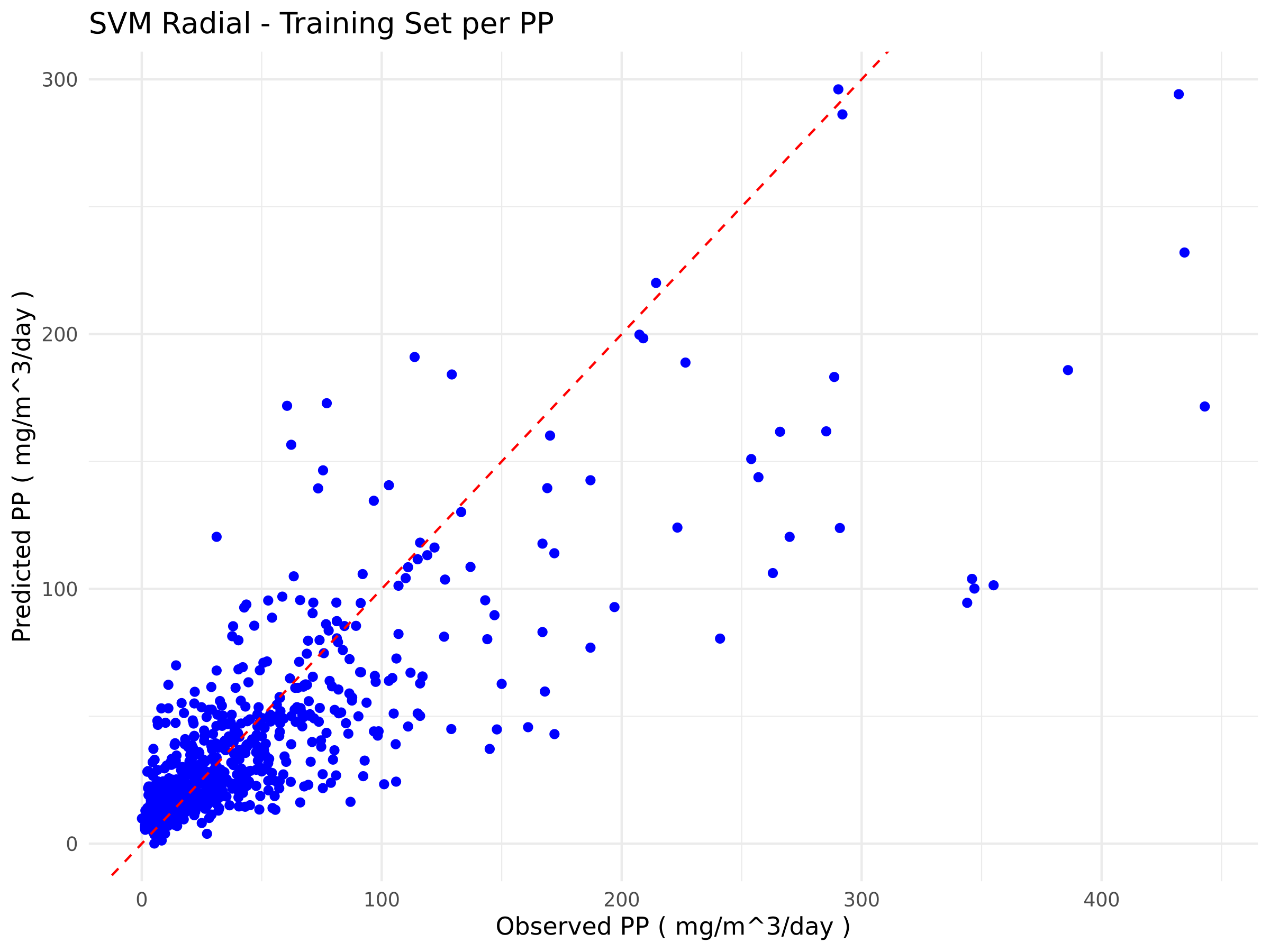
In contrast, the SVM model shows more balanced values in the training and testing phases, with R² increasing from 0.6481 to 0.7049, and errors reducing on the validation set. This consistency across the two phases suggests better generalisation and lower sensitivity to noise in the data. While XGBoost remains potentially more powerful, the current results show that SVM provides more reliable performance on the test set under the considered experimental conditions.
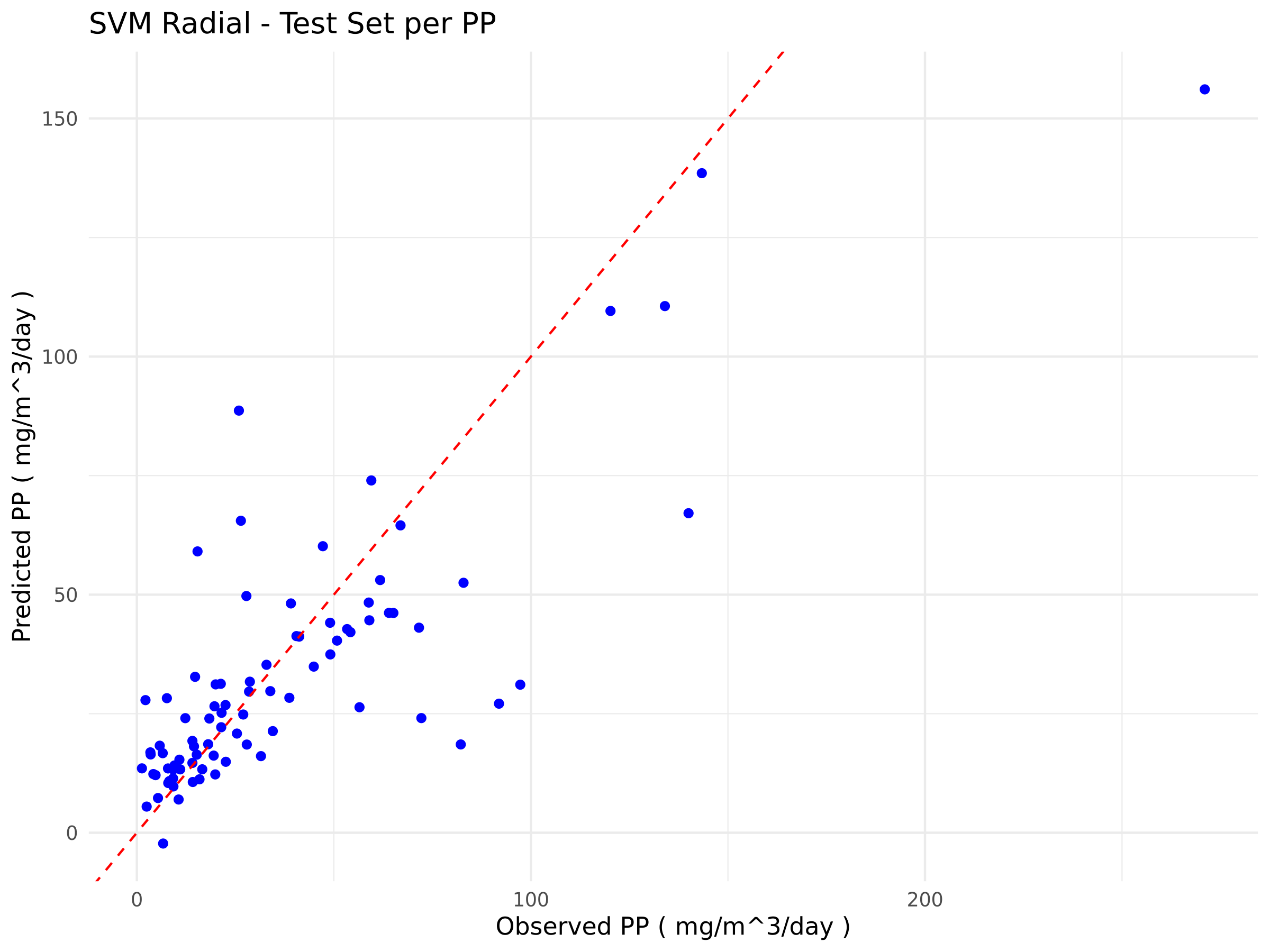
The plots below (Figure 1) show the relationship between the observed and predicted values for the best-performing algorithms in each training and testing phase for Extreme Gradient Boosting (Figure 1a) and Support Vector Machine (Figure 1b).
a)
b)
Figure 1. Scatter plots comparing observed and predicted values from the models. The blue points represent the model predictions relative to the actual data, while the red dashed line indicates the ideal 1:1 correspondence. a) Scatter plots of eXtreme Gradient Boosting; b) Scatter Plots of Support Vector Machine
This study aims to develop a machine-learning algorithm capable of making predictions based on new biotic and abiotic data, in order to evaluate the contribution of each variable to the target outcome (PP). Therefore, when choosing the best algorithm, we prioritise performance during the testing phase. Accordingly, we selected the Support Vector Machine (SVM) model, which, although it shows lower performance during training, generalises better to unseen data, that is, observations not used during training.
The SHAP analysis applied to the Support Vector Machine (SVM) model indicates that the variables with the greatest influence on the PP predictions are Chl (chlorophyll), Irr (irradiance) and SST (sea surface temperature). The SHAP bar plot for the SVM, which supports this finding, is provided among the outputs under the name ‘shap_importance_bar_plot’.
Technical notes
All the information and outputs presented in this case study were produced using the same method for each machine-learning algorithm tested. Here, we highlight only the most relevant information for this particular case study. For a full description of all WF4 outputs, please refer to the training section of the website. Essentially, if the user introduces a “Prediction” file containing the new dataset of predictors, WF4 will perform the estimation of the target variable using the best model set for each algorithm in WF4.