Use case WF 5
Effects of primary productivity and aquatic biomass on biodiversity
WF5 is designed to manage and analyze in situ geospatial monitoring data, integrating information derived from remote sensing. In particular, WF5 makes it possible to correlate aquatic biodiversity indicators and diversity indices (e.g. species richness, Shannon index, Simpson index and others) with Net Primary Productivity and/or chlorophyll-a concentration, while also incorporating abiotic variables obtained from satellite sensors and their products, as well as additional information such as distance from the coast and water depth. All analyses are performed using the same geographical sampling areas as the species abundance/richness data.
The proposed case study aims to (i) quantify the relationship between biodiversity, biotic variables, and abiotic variables, and (ii) identify spatial biodiversity hotspots within the available dataset.
Dataset
The WF5 workflow links aquatic biodiversity (in this case study expressed as species richness) to both Net Primary Productivity (NPP) and chlorophyll-a concentration (Chl-a, used as a proxy for aquatic biomass). The analysis also integrates a set of abiotic variables: sea surface temperature (SST), photosynthetically active radiation (PAR), particulate organic carbon (POC), and particulate inorganic carbon (PIC). In addition, WF5 allows the monitoring data to be associated with distance from the coast (distanceFromCoast) and water depth, with stratification based on the geographic areas from which the species richness data were collected.
NPP estimates are derived from model-based satellite products provided by Ocean Productivity (https://orca.science.oregonstate.edu/index.php). Chl-a, SST, PAR, PIC, and POC datasets are sourced from MODIS sensor products distributed via the Ocean Color platform (https://oceancolor.gsfc.nasa.gov/).
Distance from the coast is computed directly within WF5 using the coordinates of the monitoring stations (or other target locations) and a coastal shoreline shapefile (SHP). Water depth is extracted in WF5 from a bathymetric raster, again based on the coordinates of the points of interest.
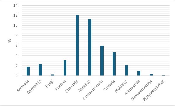
The in situ biodiversity measurements for the study area were by extrapolating and reprocessing the subset of the BioTime dataset (Figure 1)(https://biotime.st-andrews.ac.uk/).
Method
To assess the feasibility of clustering biodiversity as a function of primary productivity, the analysis was carried out in two distinct phases (running WF5 multiple times). In the first phase, the relationship between in situ species richness and a set of explanatory variables was examined: Net Primary Productivity (NPPmean), particulate inorganic carbon (PICmean), particulate organic carbon (POCmean), distance from the coast and depth. Sea surface temperature (SSTmean), chlorophyll-a (Chl-amean) and photosynthetically active radiation (PARmean) were excluded at this stage, as these are used to derive NPPmean.
In the second phase, the relationship between in situ species richness and Chl-a mean, SSTmean, PARmean, PICmean, POCmean, distanceFromCoast and depth was evaluated. NPPmean was not included in this second stage, since the focus was on the direct effect of its underlying drivers. In both phase, the workflow consists of three steps:
- Principal Component Analysis (PCA) to explore the main multivariate gradients in the environmental data.
- Regression analysis to quantify how these variables explain biodiversity patterns (species richness).
- Clustering, performed on species richness together with NPP (in the first stage) and with Chl-a (in the second stage), to identify groups of sites with similar biodiversity–productivity profiles.
Results
1) PCA of Species Richness vs. NPP, POC, PIC, Distance from the Coast, and Depth
The first two principal components account for the majority of the variability in the data. PC1 explains 78.2% of the variance, and PC2 explains a further 11.8%, giving a total of approximately 90.0% (“all_data_explained_variance”). This suggests that the dominant ‘signal’ is essentially two-dimensional (see Figure 2).
PC1 shows positive loadings for POCmean, PICmean, NPPmean and depth, as well as a negative loading for distanceFromCoast. So, PC1 scores increase in areas with higher productivity/carbon content (POCmean, PICmean and NPPmean) and greater depth, and decrease with increasing distanceFromCoast.
PC2 is mainly driven by depth (loading = 0.71), in contrast to PICmean (loading = –0.50). POCmean and offshore also have negative loadings (approximately –0.33 and –0.34, respectively), while NPPmean is only weakly negative (approximately –0.15). PC2 therefore contrasts deeper sites (high scores) with shallower sites that have higher PICmean and lie closer to the coast (low scores).
Correlations between species richness and the first two components are weak: approximately 0.093 for PC1 and approximately 0.046 for PC2. Stronger, albeit negative, correlations appear for PC3 (approximately –0.143) and particularly PC4 (approximately –0.222); PC5 is also negative (approximately –0.105). However, these higher components explain only a small fraction of the total variance compared to PC1–PC2.
This suggests that in this case study, the PCA may not be the most suitable method to capture biodiversity–environment relationships in this dataset, at least not in a strictly linear/global way.
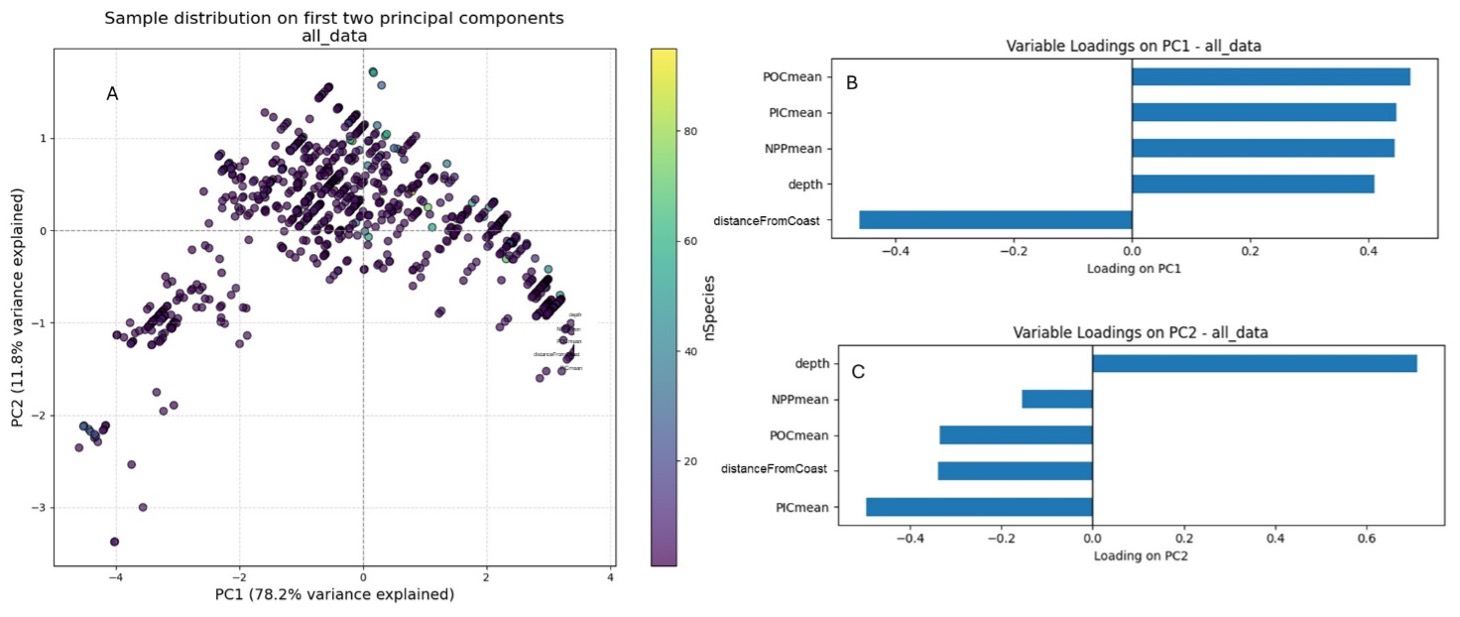
Figure 2. PCA results obtained using species richness as the target variable and NPPmean, POCmean, PICmean, distanceFromCoast, and depth as predictors. A) Biplot of PC1 vs PC2. B) Bar plot of variable loadings showing how each variable contributes to PC1. C) Bar plot of variable loadings showing how each variable contributes to PC2.
2) PCA of Species Richness vs SST, PAR, CHL-a, PIC, POC, Distance from the Coast, and Depth
The first two principal components explain the majority of the variability in the data: PC1 accounts for 61.2%, while PC2 accounts for 16.8%. Together, they account for approximately 78.0% of the variance. This indicates that the dominant signal is largely two-dimensional (Figure 3).
PC1 captures a coastal–productivity/depth gradient. It shows strong positive loadings for Chl-a mean, POCmean, PICmean and depth. SSTmean loads moderately positively, PARmean loads weakly positively, and distance from the coast loads negatively. In practical terms, PC1 scores are higher in waters that are more productive (higher concentrations of Chl-a mean, POCmean and PICmean), deeper and closer to the coast.
PC2 reflects a light-and-temperature gradient. It is characterised by strong positive loadings for PARmean (approximately 0.82) and SSTmean (approximately 0.53), as well as a smaller positive contribution from distance from the coast (approximately 0.15). The remaining variables have small or slightly negative loadings. PC2 therefore separates environments with high irradiance and warmer surface waters from cooler, lower-light environments.
Correlations between species richness and the first two components are weak: approximately 0.112 for PC1 and approximately –0.119 for PC2. The strongest correlation emerges with PC3 (approximately 0.261), while PC4–PC7 show lower values. Since PC3 and PC4 each explain a smaller proportion of the total variance (9.7% and 9.5%, respectively), this suggests that variation in species richness is primarily captured by subsequent environmental gradients.
This suggests that in this case study, the PCA may not be the most suitable method to capture biodiversity–environment relationships in this dataset, at least not in a strictly linear/global way.

Figure 3. PCA results obtained using species richness as the target variable and NPPmean, POCmean, PICmean, distanceFromCoast, and depth as predictors. A) Biplot of PC1 vs PC2. B) Bar plot of variable loadings showing how each variable contributes to PC1. C) Bar plot of variable loadings showing how each variable contributes to PC2.
Regression
To better characterise the relationships between species richness and the selected predictor variables, we employed a regression approach. As a standard linear regression did not yield reliable results, we adopted a non-linear model: Random Forest.
The Random Forest model, which used species richness vs NPPmean, POCmean, PICmean, distanceFromCoast and depth as predictors, was trained using a hold-out validation strategy. This model demonstrates reasonable generalisation performance, with a test R² of 0.584, an RMSE of around 5 and an MAE of around 3 (Figure 4). The observed train–test discrepancy indicates moderate overfitting, which aligns with the model’s high flexibility.
Permutation importance analysis (ΔR²) reveals a clear hierarchy of predictors. distanceFromCoast is by far the most informative variable, followed by depth, POCmean and PICmean. NPPmean contributes little to the model’s predictive ability. Overall, coastal gradients and the biogeochemical properties of the water column emerge as the key drivers of species richness.

Figure 4. A) Relationship between predicted and observed values in the training phase of the model. B) Relationship between predicted and observed values in the test phase of the model. C) Ranked variable importance in the model.
The Random Forest model, which used species richness vs SSTmean, PARmean, Chl-a mean, PICmean, POCmean, distanceFromCoast and depth, as predictors, was trained using a hold-out validation strategy. This model demonstrates reasonable generalisation performance, with a test R² of 0.511, an RMSE of around 6 and an MAE of around 3 (Figure 5). Compared to the training set (R² = 0.884), this suggests some overfitting, which is consistent with the flexibility of the algorithm.
Permutation importance analysis (ΔR²) reveals a clear ranking of the importance of the predictors. Distance from the coast (offshore) is by far the most informative variable, followed by mean Chl-a mean, then depth, POCmean, PICmean, PARmean and SSTmean. Mainly, SSTmean appears to add little or no additional predictive power to the model. These results suggest that, in this dataset, distanceFromCoast and productivity proxies, such as Chl-a mean, are the main predictors of species richness.

Figure 5. A) Relationship between predicted and observed values in the training phase of the model. B) Relationship between predicted and observed values in the test phase of the model. C) Ranked variable importance in the model.
Clustering
In this case study, PCA is not effective at discriminating the contribution of individual variables to biodiversity, likely because the relationship between the response variable (species richness) and the predictor variables is nonlinear. In contrast, the Random Forest model can capture these nonlinearities and highlights the significant contribution of Chl-a mean to predictions.
Based on this, we can cluster biodiversity according to Chl-a mean concentration, which is used here as a proxy for aquatic biomass. Figure 6 shows the resulting biodiversity clusters in relation to Chl-a mean concentration. Clusters with higher species richness tend to be located close to the coast in shallower areas.

Technical notes
The workflow is flexible and adaptable in terms of how the target and predictor variables are defined. Users can select the variables to include according to their specific objectives.
In this case study, clustering was performed by examining the relationship between Y (species richness) and one X variable at a time (either NPPmean or Chl-a mean). However, clustering can also be performed using multiple X variables simultaneously or based on Y alone. Further details can be found in the training section.