Use case WF 6
Environmental Regulation of Chlorophyll and Primary Production Across the Adriatic and Ionian Seas
The workflow allows for the modelling of multiple dependent variables (Y) as a function of several independent variables (X). In the context of VRE Biomass, this approach facilitates analysis of the intricate relationships between biotic and abiotic factors.
This case study aims to identify the main environmental drivers that control the functioning of the productive system within the study area and to assess how they influence system productivity, with a particular focus on the combined effects of abiotic factors on phytoplankton biomass (chlorophyll) and Primary Productivity (PP). Redundancy Analysis (RDA) was employed to quantify and visualise the relationships between biotic response variables and environmental covariates. Subsequently, univariate ANCOVA models were developed to determine the specific contributions of these drivers to each response variable and to test for potential interactions between factors and covariates. Overall, the objective of this study is to evaluate the relative influence of abiotic drivers on total primary production (PP and Chl) in the Adriatic and Ionian Seas, and to determine whether the relationships between key environmental factors and system productivity exhibit basin-specific patterns.
Dataset
The dataset includes abiotic (physico-chemical parameters and nutrients) and biotic (chlorophyll and primary production, fractionated by size classes) measurements collected at different marine stations in two basins: the Adriatic and Ionian Seas in the 2000. For the analyses conducted in this study, only measurements acquired at zero depth were considered.
The X and Y variables used in the analyses are as follows:
- Predictor variables (X): Temperature, dissolved oxygen (DO), salinity, ammonium, nitrate, nitrite, silicate and DIP.
- Target variables (Y): Total chlorophyll (Chl tot) and total primary production (PP tot).
Additional details about the dataset used in this use case are publicly available through the LifeWatch Italy metadata catalogue at the following link: https://metadatacatalogue.lifewatchitaly.eu/geonetwork/srv/eng/catalog.search#/metadata/c66df408-917b-499a-a942-a28c2553aa7d.
Method
The predictor matrix was defined based on a specification file (Parameter.csv), which identified the response variables (Y), continuous covariates (X) and categorical factors (F).
The environmental variables (Temperature, DO, Salinity, Ammonium, Nitrate, Nitrite, Silicate and DIP) used in the analyses were standardised using z-scores. The biotic variables (Chl tot and PP tot) included in the RDA and ANCOVA were log-transformed using a base-10 logarithm with a unit pseudocount (log₁₀(1 + Y)) to avoid issues related to potential zero values.
The analyses were performed using multicollinearity among the abiotic variableswith an iterative approach based on the variance inflation factor (VIF). The VIF was calculated for all numerical X variables and a maximum threshold of 5 was applied to remove potentially collinear predictors.
RDA was used to identify the common multivariate pattern and the main environmental gradient governing the system as a whole. Redundancy analysis (RDA) was implemented in Python. In the RDA workflow, as all transformations had already been applied to the final dataset, no additional scaling was performed on the X variables during the analysis. Instead, the log-transformed Y variables were centred (zero mean per column). The centred response matrix Y was then projected onto the space defined by the scaled X variables through multivariate regression to yield the constrained values Ŷ. PCA was then performed on Ŷ to obtain sample scores, biotic variable loadings and eigenvalues. The variance explained by the RDA axes was expressed relative to the total inertia of Y. Both R² and adjusted R² were calculated using the formulation commonly adopted in multivariate ecology. Model significance was assessed via permutation testing (999 permutations) by permuting the rows of Y to generate a null distribution, then comparing the observed F-value with the permuted values. Finally, the association between the environmental variables and the RDA axes was estimated by calculating the Pearson correlation coefficient between each X variable and the scores of the first two axes. These correlations were then used to construct the final biplot, displaying samples alongside biotic and abiotic vectors.
ANCOVA was used to determine, for each biotic variable, which drivers are significant, quantify the strength of their effects, and assess whether these effects differ between groups. As all the necessary transformations had already been incorporated into the dataset, no additional scaling was applied to the covariates in the ANCOVA. To estimate the main effects while controlling for non-orthogonality among the predictors, sum-to-zero contrasts and Type III tests were used in the analysis, which is an appropriate approach for designs that are not perfectly balanced. An OLS model in ANCOVA form was then fitted for each biotic response variable. Since ecological relationships with environmental gradients may vary across factor levels, the presence of factor × covariate interactions was assessed. These interactions were only retained if they were statistically significant (p < 0.05); otherwise, a more parsimonious reduced model was preferred. A hierarchical backward selection procedure based on the Bayesian Information Criterion (BIC) was subsequently applied to the selected formula (full or reduced), favouring clearer models and avoiding overfitting. Finally, post hoc analyses were performed using Estimated Marginal Means (EMMs), with pairwise comparisons and Holm-adjusted p-values, when significant or biologically relevant factors were present in the final model.
RDA analysis
The application of the VIF did not result in the removal of any variables, as no problematic multicollinearity was detected among the covariates used in the analysis.
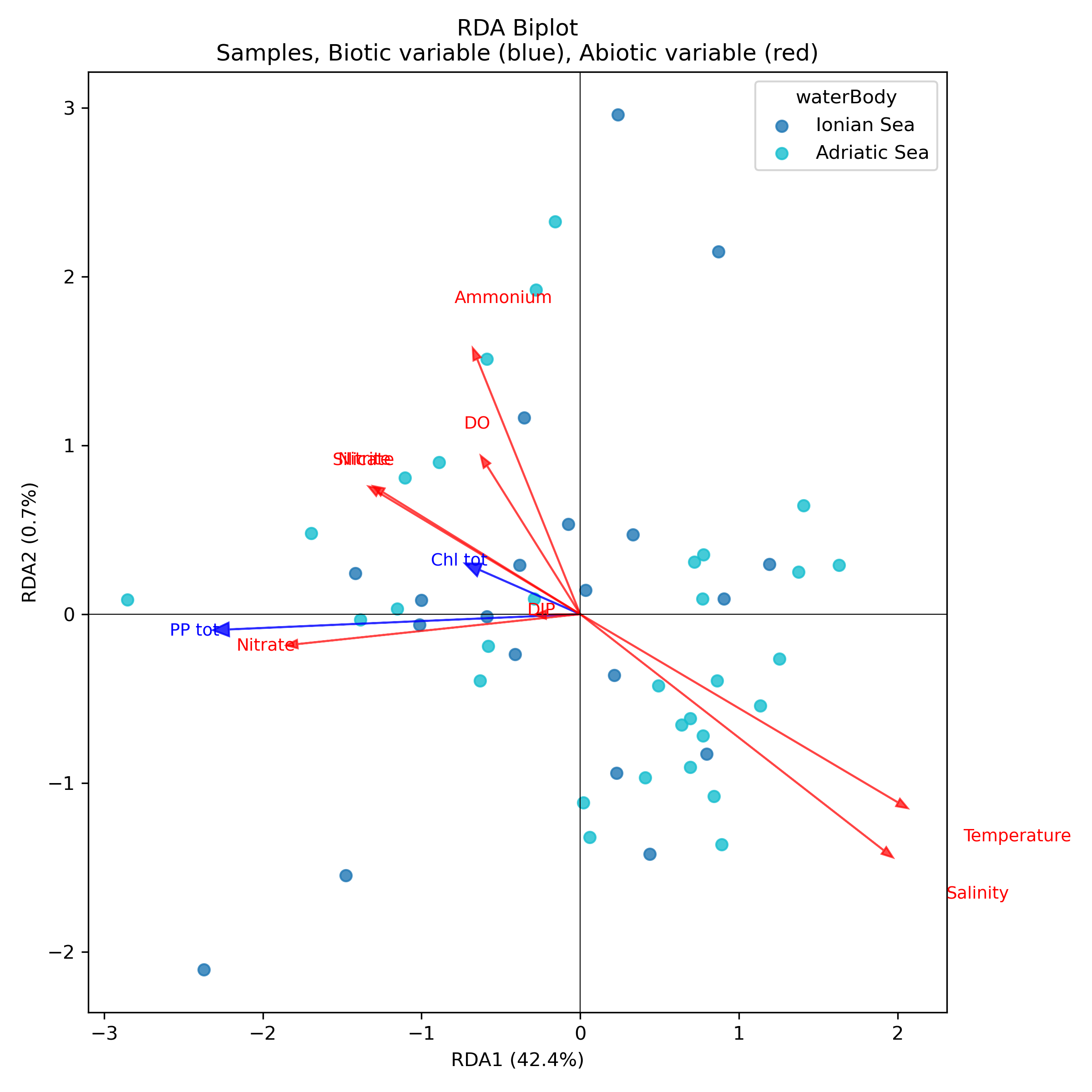
Redundancy analysis (RDA) revealed a strong environmental gradient capable of explaining a substantial proportion of the observed biotic variability. The constrained axes collectively accounted for 42.18% of the total variance in the biotic responses, with the first axis showing clear dominance. In this study, considering the dataset that was used, RDA1 explained 42,4% of the variance, while RDA2 accounted for just 0.7%, suggesting that almost all the relevant ecological structure is captured by the primary gradient. A global permutation test confirmed the significance of both the model (p < 0.05) and the first axis (p < 0.05), while RDA2 was not significant (p > 0.05). This supports the interpretation of a single dominant ecological dimension. This highly imbalanced distribution suggests the existence of a primary ecological gradient, which is almost entirely captured by the first RDA1, with minimal contribution from the RDA2. The RDA biplot (Figure 1) reveals a clear directional structure among the environmental variables. The vectors for salinity and temperature are long and strongly aligned along RDA1, suggesting that these are the primary abiotic factors responsible for the observed biological variation. Nutrients (nitrate, silicate and ammonium) also contribute positively to the ordination, but their vectors are considerably shorter than those of the thermohaline variables, suggesting an additional, albeit less pronounced, influence. Dissolved oxygen (DO) occupies an intermediate position along RDA1, which is consistent with the secondary role of the other chemical parameters of the water.
The biotic variables exhibit differentiated response patterns. Total primary production (PP_(tot)) is negatively oriented along RDA1, indicating a decline in biological productivity with increasing temperature and salinity (Table 1). Total chlorophyll (Chl_(tot)) shows a partial association with RDA2. However, as this axis only accounts for a very small fraction of the variance (<1%), this pattern should be interpreted with caution. This suggests that chlorophyll may be modulated by more local factors or residual variability not explained by the model, rather than responding strongly to the main environmental gradients.
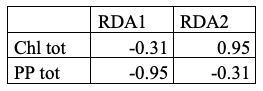
Table 1. Loadings (correlation/projection coefficients) of the biotic variables on the first two axes of Redundancy Analysis (RDA).
In our case study, although the RDA captures less than 50% of the variance, the RDA results suggest that biotic structure is primarily determined by two key environmental factors: salinity and temperature. Nutrients also influence this structure, albeit to a lesser extent. The alignment of biological responses with these gradients lends weight to the notion that the physicochemical conditions of the water are the primary determinants of productivity and biotic composition in these aquatic ecosystems. These dynamics are consistent with reports in the literature on coastal and shelf systems subject to significant thermohaline variability.
ANCOVA analysis
Having explored the multivariate structure of the biological responses and their overall association with environmental gradients using RDA, we examined the identified relationships further using ANCOVA. Specifically, we used ANCOVA to inferentially test the effects of individual abiotic covariates and the basin factor (water body) on each biotic variable, while also assessing potential differences in slopes (factor × covariate interactions). This complementary approach allows us to transition from an ordination-based description of global patterns (RDA) to a statistical quantification of effects and basin-specific responses while controlling for the main environmental drivers simultaneously.
CHL-a
The fixed-effects ANCOVA (Type III) on total chlorophyll concentration (Chl tot) indicates that the statistical model adopted (OLS) adequately describes the observed variability. The final model has an R² of 0.678 (adjusted R² = 0.626) and is significantly better than the null model (F = 12.95, p = 8.06×10⁻⁹). Residual diagnostics confirm that the main assumptions of the linear model are met: residuals are normally distributed (Shapiro–Wilk p = 0.8616), and no evidence of heteroscedasticity emerges (Breusch–Pagan p = 0.8336). Overall, these results support the robustness of the statistical inference (Fig. 2a).
Examination of the coefficients shows a significant main effect of temperature, which is negatively associated with total Chl tot (β = −0.0142; p = 0.016). Silicate also exhibits a positive main association with total Chl (β = 0.0121; p = 0.044), whereas salinity and nitrite are not significant as main effects. However, significant interactions emerge between water body and some chemical variables: specifically, the water body × salinity interaction is negative (β = −0.0153; p = 0.049), the water body × nitrite interaction is positive (β = 0.0189; p = 0.002), and the water body × silicate interaction is negative (β = −0.0184; p = 0.004). These interactions indicate that the effect of these nutrients on total chlorophyll varies depending on the basin considered.
The estimated marginal means (EMMs) of Chl tot are very similar between the Adriatic and Ionian Seas, with substantial overlap of the 95% confidence intervals. This indicates the absence of a main effect of water body on Chl tot once environmental covariates are controlled for. (Figure 2). This does not imply that the two systems respond in the same way to environmental factors.
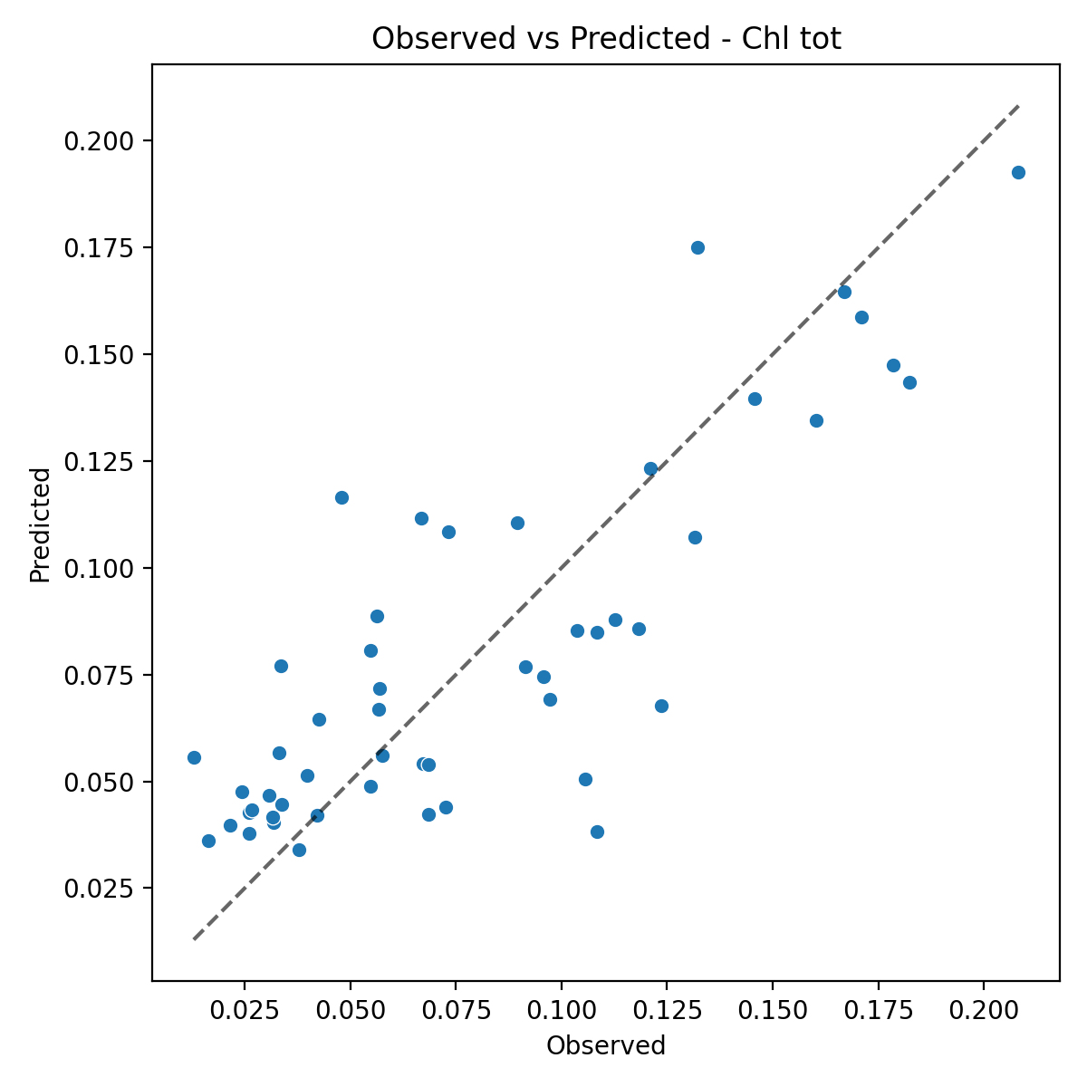
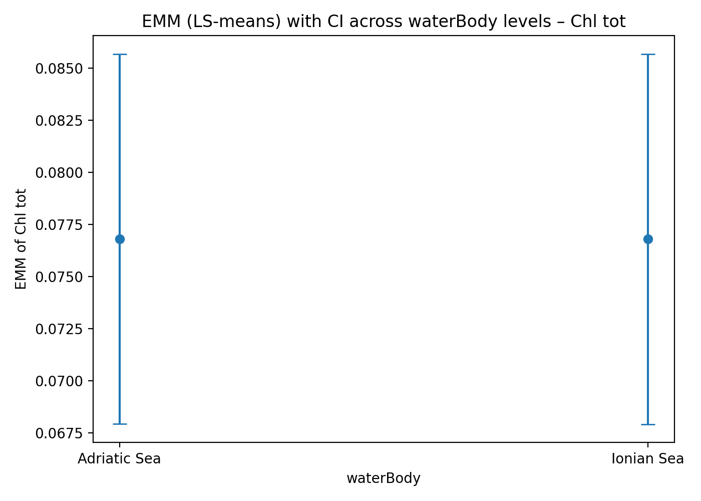
Figure 2. (a) Relationship between observed values and ANCOVA-predicted values for Chl tot. (b) Estimated Marginal Means (EMMs) of total chlorophyll in the two basins (Adriatic Sea and Ionian Sea), with 95% confidence intervals.
However, the response of chlorophyll to environmental factors is not uniform across the two systems. In particular, significant interactions between waterBody and nutrient concentrations (salinity, nitrite and silicate) suggest that the relationship between nutrients and Chl tot differs consistently between the two seas (Figure 3). This reveals that the two ecosystems have different ecological sensitivities to nutrient variations, indicating that the effect of salinity, silicate and nitrate on Chl tot is modulated by the basin context. This difference could reflect specific eco-hydrodynamic and biogeochemical characteristics of the two seas that are not explicitly represented in the model covariates.

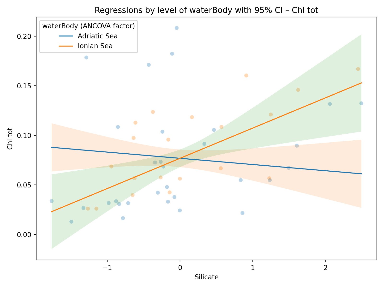

Figure 3. Relationships between environmental variables and Chl tot in the two basins considered. (a) Salinity, (b) Silicate, and (c) Nitrite.
PP
The ANCOVA performed on total primary production (PP tot) shows that the OLS model explains a moderate but statistically significant portion of the observed variability (R² = 0.497; adjusted R² = 0.415) and performs substantially better than the null model (F = 6.058, p = 5.97×10⁻⁵).Residual diagnostics confirm that the main assumptions of the linear model are met: residuals are normally distributed (Shapiro–Wilk p = 0.1375), and no evidence of heteroscedasticity emerges (Breusch–Pagan p = 0.5179). Overall, these results support the robustness of the statistical inference.
Among the environmental covariates, PP tot shows a significant negative relationship with ammonium (β = −0.1191, p = 0.002) and significant positive relationships with nitrate (β = 0.0766, p = 0.001) and nitrite (β = 0.0797, p = 0.023). Salinity exhibits only a marginal negative trend (p = 0.067), while silicate is not associated with PP tot as a main effect (p = 0.126). A significant waterBody × Ammonium interaction is also present (β = 0.0832, p = 0.003), indicating a differential productivity response to ammonium between the two basins. In contrast, the waterBody × Silicate interaction is significant and negative (β = −0.0561, p = 0.017), showing that the effect of silicate on PP tot varies between water bodies, with the sign of the relationship changing across basins.
The estimated marginal means (EMMs) of PP tot are very similar between the Adriatic and Ionian Seas, with substantial overlap of the 95% confidence intervals. This indicates the absence of a main effect of water body on PP tot once environmental covariates are controlled for (Figure 4). This does not imply that the two systems respond in the same way to environmental factors.
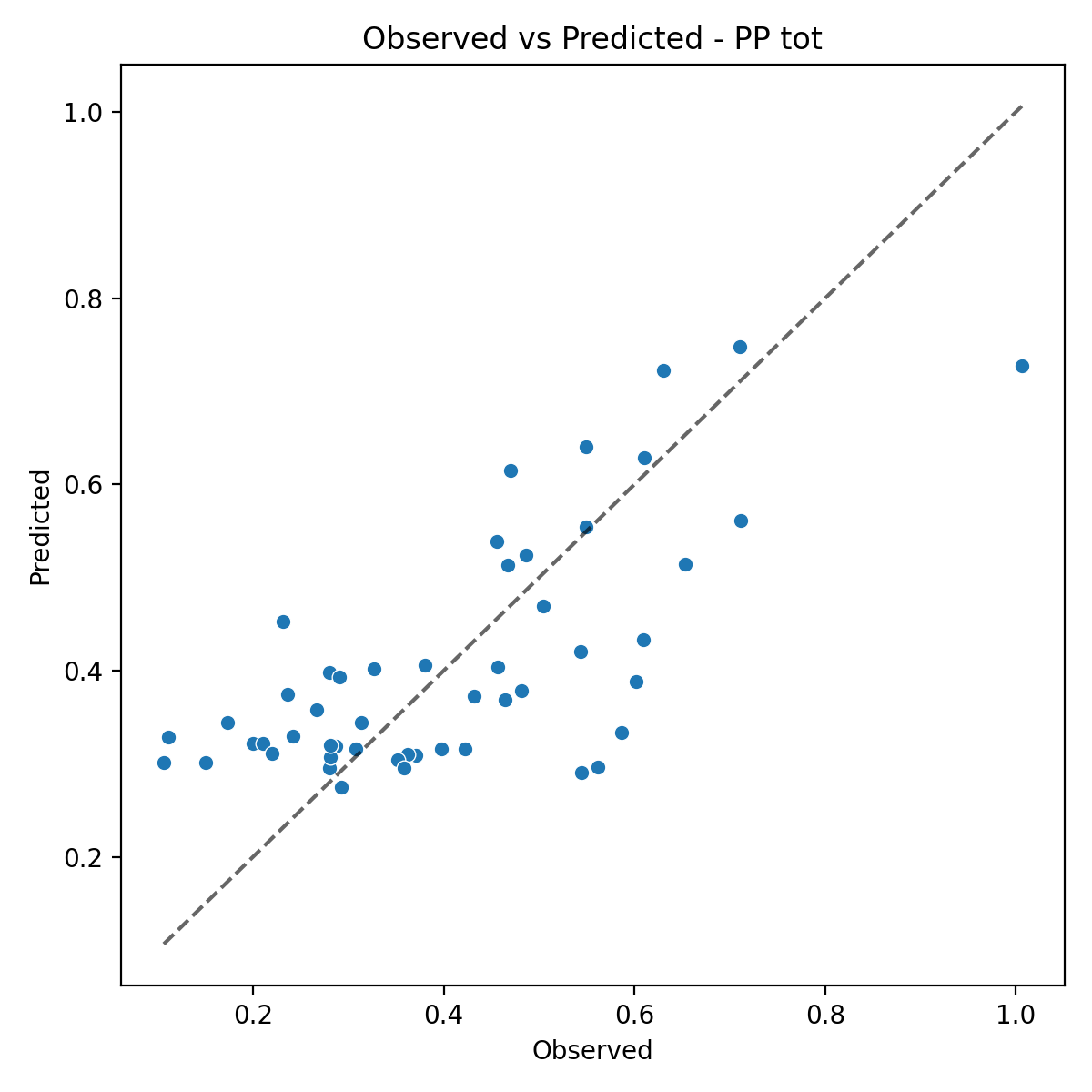
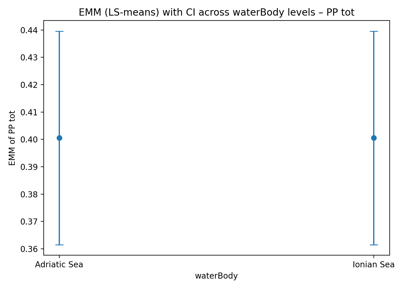
Figure 4. (a) Relationship between observed values and ANCOVA-predicted values for PP tot. (b) Estimated Marginal Means (EMMs) of total chlorophyll in the two basins (Adriatic Sea and Ionian Sea), with 95% confidence intervals.
However, the response of PP tot to environmental factors is not uniform across the two systems. In particular, significant interactions between waterBody and nutrient concentrations (ammonium and silicate) suggest that the relationship between nutrients and PP tot differs consistently between the two seas (Figure 5). This reveals that the two ecosystems have different ecological sensitivities to nutrient variations, indicating that the effect of ammonium and silicate on PP tot is modulated by the basin context. This difference could reflect specific eco-hydrodynamic and biogeochemical characteristics of the two seas that are not explicitly represented in the model covariates.


Figure 5. Relationships between environmental variables and PP tot in the two basins considered. (a) silicate and (b) ammonium.
Technical notes
These results are consistent with the default WF6 configuration. The analysis could be further refined by adjusting the settings of individual procedures. Therefore, users can customise the analysis according to their research objectives and the level of detail they require.